Best Audio Data | Audio/Voice Data analysis Using Deep Learning

Audio Data facts evaluation the use of Deep studying with Python 

Audio Data. In recent times, deep getting to know is more and more used for tune style class: particularly Convolutional Neural Networks (CNN) taking as entry a spectrogram considered as an picture on that are sought specific forms of shape. Convolutional Neural Networks (CNN) are very just like regular Neural Networks: they're made from neurons which have learnable weights and biases. every neuron receives a few inputs, performs a dot product and optionally follows it with a non-linearity. The whole community still expresses a single differentiable score characteristic: from the raw photograph pixels on one give up to elegance ratings at the opposite. and that they still have a loss characteristic (e.g. SVM/Softmax) on the final (completely-related) layer and all of the tips/hints we evolved for gaining knowledge of regular Neural Networks still observe. So what changes? ConvNet architectures make the specific assumption that the inputs are pics, which allows us to encode sure residences into the structure. these then make the ahead feature extra green to put in force and hugely reduce the variety of parameters within the network.

Parentsource

They are able to detecting number one features, which can be then combined by next layers of the CNN architecture, ensuing within the detection of higher-order complicated and applicable novel capabilities. The dataset includes a thousand audio tracks every 30 seconds lengthy. It consists of 10 genres, every represented through 100 tracks. The tracks are all 22050 Hz monophonic sixteen-bit audio documents in .Wav layout. The dataset may be down load from marsyas internet site. It consists of 10 genres i.e

1. Blues
2. Classical
3. us of a
4. Disco
5. Hiphop
6. Jazz
7. metal
8. Pop
9. Reggae
10. Rock

Every style incorporates a hundred songs. general dataset: one thousand songs. Before shifting in advance, i might advocate using Google Colab for doing the whole lot associated with Neural networks because it's miles free and presents GPUs and TPUs as runtime environments. Convolutional Neural network implementation So allow us to begin building a CNN for genre type. first of all load all the required libraries.

• import pandas as pd import numpy as np
• importar numpy como np from numpy import argmax
• de numpy importar argmax import matplotlib.pyplot as plt
• importar matplotlib.pyplot como plt %matplotlib inline
• %matplotlib import booksa
• import online librosa import librosa.display
• import librosa.display import IPython.display
• import IPython.display import import warnings import random

Random import OS from PIL import photo import pathlib import csv # sklearn Preprocessing from sklearn .Model_selection import train_test_split #Keras import keras import warnings warnings.filterwarnings('forget') from keras import layers from keras.layers import Activation, Dense, Dropout, Conv2D, Flatten, MaxPooling2D, GlobalMaxPooling2D, GlobalAveragePooling1D, AveragePooling2D, join, aggregate from keras.models import Sequential from keras.optimizers import SGD from keras.models import Sequentialfrom keras.optimizers import SGDNow convert the audio statistics files into PNG format images or essentially extracting the Spectrogram for each Audio. we can use librosa python library to extract Spectrogram for every audio file. Genres = 'blues classical us of a disco hiphop jazz metal pop reggae rock'.split() for g in genres: pathlib.direction(f'img_data/g').mkdir(parents=proper, exist_ok=actual) for filename in os.listdir(f'./pressure/My power/genres/g'): songname = f'./power/My force/genres/g/filename' y, sr = librosa.load(songname, mono=real, period=five) print(y.shape) plt.specgram(y, NFFT=2048, Fs=2, Fc=zero, noverlap=128, cmap=cmap, sides='default', mode='default', scale='dB'); plt.axis('off'); plt.savefig(f'img_data/g/filename[:-3].replace(".", "").png') plt.clf() The above code will create a directory img_data containing all the snap shots labeled within the style.

• discernpattern spectrograms of Disco, Classical, Blues and u . s . style respectively.
• Disco and Classical
• Blues and u . s .

Our subsequent step is to cut up the facts into the train set and check set.

• installation break up-folders.
• pip install break up-folders
• we can cut up facts via eighty% in training and 20% inside the test set.
• import cut up-folders

# To simplest cut up into education and validation set, set a tuple to `ratio`, i.e, `(.eight, .2)`. split-folders.ratio('./img_data/', output="./information", seed=1337, ratio=(.eight, .2)) # default values The above code returns 2 directories for educate and check set interior a determine listing.

Picture Augmentation:

Image Augmentation artificially creates training pics through extraordinary methods of processing or aggregate of a couple of processing, together with random rotation, shifts, shear and flips, and so forth. Carry out picture Augmentation in place of education your version with masses of pix we are able to teach our model with fewer pix and schooling the version with exceptional angles and modifying the pics. Keras has this ImageDataGenerator elegance which lets in the customers to carry out photograph augmentation on the fly in a completely smooth manner. you could examine about that during Keras’s authentic documentation.

• from keras.preprocessing.photo import ImageDataGenerator train_datagen = ImageDataGenerator(
• train_datagen = ImageDataGenerator( rescale=1./255, # rescale all pixel values from zero-255, so aftre this step all our pixel values are in range (0,1)
• rescale=1./255, # rescales all pixel values ​​from zero to 255, so after this step all our pixel values ​​are in the range (0,1) shear_range=zero.2, # to use some random transformations
• shear_range=zero.2 , #to use some random transformations zoom_range=0.2, #to apply zoom
• zoom_range=0.2, #para aplicar zoom horizontal_flip=true) # image can be flipper horiztest_datagen = ImageDataGenerator(rescale=1./255)
• horizontal_flip=true) # image can be flipper horiztest_datagen = ImageDataGenerator(rescale=1./255)

The ImageDataGenerator class has 3 strategies flow(), flow_from_directory() and flow_from_dataframe() to study the pictures from a huge numpy array and folders containing images. we can speak only flow_from_directory() on this weblog post. training_set = train_datagen.flow_from_directory( './facts/educate', target_size=(64, sixty four), batch_size=32, class_mode='express', shuffle = false)test_set = test_datagen.flow_from_directory( './records/val', target_size=(sixty four, 64), batch_size=32, class_mode='categorical', shuffle = fake )

flow_from_directory() has the subsequent arguments.

listing: direction where there exists a folder, beneath which all of the take a look at pix are present. for example, in this example, the training photographs are determined in ./facts/teach batch_size: Set this to a few quantity that divides your total variety of pictures to your check set precisely. Why this simplest for test_generator?

Why is this simpler for test_generator?

actually, you have to set the “batch_size” in each teach and valid turbines to a few wide variety that divides your total wide variety of images for your teach set and valid respectively, however this doesn’t be counted earlier than because although batch_size doesn’t suit the wide variety of samples in the teach or legitimate sets and a few snap shots gets overlooked out every time we yield the pix from generator, it'd be sampled the very subsequent epoch you educate. however for the check set, you ought to pattern the snap shots precisely as soon as, no much less or no more. If puzzling, simply set it to one(however perhaps a little bit slower). class_mode: Set “binary” if you have simplest lessons to are expecting, if not set to“specific”, in case in case you’re developing an Autoencoder device, each input and the output could possibly be the identical image, for this case set to “input”. shuffle: Set this to false, due to the fact you need to yield the snap shots in “order”, to predict the outputs and match them with their particular ids or filenames.

Create a Convolutional Neural network:

• version = Sequential() input_shape=(sixty four, sixty four, three)#1st hidden layer
• input_shape=(sixty-four, sixty-four, three)#1st model.add(Conv2D(32, (3, three), strides=(2, 2), input_shape=input_shape))
• modelo de capa oculta.add(Conv2D(32, (3, tres), strides=(2, 2), input_shape=input_shape)) version.add(AveragePooling2D((2, 2), strides=(2,2)))
• version.add (AveragePooling2D((2, 2), strides=(2,2))) model.add(Activation('relu'))#2d hidden layer
• model.add(Activation('relu'))#2d model.upload(Conv2D(sixty four, (three, three), padding="same"))
• hidden layer model.upload(Conv2D(sixty-four, (three, three), padding= "same")) version.add(AveragePooling2D((2, 2), strides=(2,2)))
• version.add(AveragePooling2D((2, 2), strides=(2,2))) version.add(Activation('relu'))#3rd hidden layer
• version.add(Activation('relu'))#3er model.upload(Conv2D(sixty four, (3, 3), padding="same"))
• hidden layer model.upload(Conv2D(sixty-four, (3, 3), padding="same")) model.add(AveragePooling2D((2, 2), strides=(2,2)))
• model.add(AveragePooling2D((2, 2), strides=(2,2))) model.add(Activation('relu'))#Flatten
• model.add(Activation('relu'))#Flatten model.upload(Flatten())
• model.upload (Flatten()) model.upload(Dropout(price=zero.5))#add absolutely connected layer.
• model.upload(Dropout(price=zero.5))#add absolutely connected layer. model.add(Dense(64))
• model.add(Dense(64)) version.upload(Activation('relu'))
• version.upload(Activación('relu')) version.upload(Dropout(rate=0.five))#Output layer
• version.upload(Drop(rate=0.five))#Output layer version.add(Dense(10))
• version.add(Dense(10)) model.upload(Activation('softmax'))model.precis()
• model.upload(Activation ('softmax'))model.precis()

bring together/train the network the use of Stochastic Gradient Descent(SGD). Gradient Descent works exceptional while we've got a convex curve. however if we don’t have a convex curve, Gradient Descent fails. therefore, in Stochastic Gradient Descent, few samples are selected randomly rather than the whole data set for each generation.

• epochs = two hundred batch_size = 8
• batch_size = 8 learning_rate = zero.01
• learning_rate = zero.01 decay_rate = learning_rate / epochs
• decay_rate = learning_rate / momentum = 0.9
• impulso de épocas = 0.9 sgd = SGD(lr=learning_rate, momentum=momentum, decay=decay_rate, nesterov=false)
• sgd = SGD(lr=learning_rate, momentum=momentum, decay=decay_rate, nesterov=false) model.compile(optimizer="sgd", loss="categorical_crossentropy", metrics=['accuracy'])
• model.compile(optimizer="sgd", pérdida="categorical_crossentropy", métricas=['exactitud'])

Now in shape the model with 50 epochs.

• version.fit_generator( training_set,
• training_set, steps_per_epoch=one hundred,
• steps_per_epoch=one hundred, epochs=50,
• epochs=50, validation_data=test_set,
• validation_data=test_set, validation_steps=2 hundred)
• validation_steps=200)

Now for the reason that CNN model is skilled, allow us to examine it. evaluate_generator() uses both your check input and output. It first predicts output the use of training input after which evaluates the performance by way of comparing it towards your check output. So it offers out a measure of overall performance, i.e. accuracy in your case. #version evaluation model.evaluate_generator(generator=test_set, steps=50)#OUTPUT [1.704445120342617, 0.33798882681564246]

So the loss is 1.70 and Accuracy is 33.7%.

At remaining, permit your version make a few predictions on the take a look at data set. You want to reset the test_set before each time you call the predict_generator. that is critical, if you forget to reset the test_set you may get outputs in a unusual order. test_set.reset() pred = model.predict_generator(test_set, steps=50, verbose=1) As of now predicted_class_indices has the anticipated labels, but you can’t really tell what the predictions are, due to the fact all you could see is numbers like 0,1,4,1,zero,6… You need to map the predicted labels with their precise ids inclusive of filenames to find out what you predicted for which photograph.

• predicted_class_indices=np.argmax(pred,axis=1)
• labels = (training_set.class_indices) labels = dict((v,okay) for ok,v in labels.items())
• labels = dict((v,okay) for ok,v in labels.items()) predictions = [labels[k] for k in predicted_class_indices]
• predictions = [tags[k] for k in predicted_class_indices] predictions = predictions[:200]
• predictions = predictions[:200] filenames=test_set.filenames
• filenames =test_set. file names

Append filenames and predictions to a single pandas dataframe as two separate columns. but before doing that check the dimensions of both, it should be the equal. print(len(filename, len(predictions))) # (200, 2 hundred) subsequently, save the outcomes to a CSV record. outcomes=pd.DataFrame("Filename":filenames, "Predictions":predictions,orient='index') effects.to_csv("prediction_results.csv",index=false) parentOutput i have trained the model on 50 epochs(which itself took 1.five hours to execute on Nvidia K80 GPU). in case you wanna boom the accuracy, growth the variety of epochs to one thousand or even more while education your CNN version. So it indicates that CNN is a viable opportunity for computerized function extraction. Such discovery lends help to our hypothesis that the intrinsic traits in the variation of musical data are just like the ones of photo facts. Our CNN model is exceptionally scalable but no longer strong sufficient to generalized the education result to unseen musical information. this will be conquer with an enlarged dataset and of direction the quantity of dataset that may be fed. properly, this concludes the 2-article series on Audio statistics evaluation the use of Deep studying with Python. i hope you men have loved studying it, feel unfastened to percentage your comments/mind/remarks in the comment section. Audio document Processing: ECG Audio the use of Python basics of Audio record Processing in R   growing a web utility to Extract subjects from Audio with Python Bark: The ultimate Audio generation version

• Bark: the definitive version of audio generation WavJourney: A adventure into the world of Audio Storyline generation
• WavJourney: an adventure in the world of high performance audio Deep gaining knowledge of, component 1
• High performance Storyline generation Deep knowledge acquisition of component 1, excessive-overall performance Deep mastering: the way to train smaller, quicker, and…
• high- overall performance Deep mastering: how to educate smaller, faster , and…
• High Performance Overall Deep Mastering: How to Educate the Smallest, Fastest, and…

We live within the world trendy sounds: quality and worrying, low and excessive, quiet and loud, they effect our mood and our decisions. Our brains are constantly processing sounds to give us essential statistics approximately our environment. however acoustic alerts can inform us even greater if analyze them the use of cutting-edge technology. today, we've AI and system contemporary to extract insights, inaudible to humans, from speech, voices, loud night breathing, track, business and visitors noise, and other modern day acoustic alerts. In this article, we’ll share what we’ve found out while creating AI-based totally sound reputation solutions for healthcare projects. specifically, we’ll give an explanation for the way to gain audio facts, prepare it for analysis, and select the right ML model to attain the highest prediction accuracy. but first, let’s go over the basics: what's the audio analysis, and what makes audio records so difficult to address. what is audio analysis?

What is audio analysis?

Audio analysis is a process of remodeling, exploring, and decoding audio indicators recorded by means of virtual devices. Aiming at information sound statistics, it applies a number of technology, inclusive of 49a2d564f1275e1c4e633abc331547db deep present day algorithms. Audio analysis has already received wide adoption in various industries, from amusement to healthcare to manufacturing. below we’ll provide the maximum popular use cases. Speech reputation

Speech reputation

La Speech popularity is about the capacity cutting-edge computers to differentiate spoken phrases with herbal language processing techniques. It allows us to govern pcs, smartphones, and different devices via voice commands and dictate texts to machines as opposed to manual entering. Siri by means of Apple, Alexa with the aid of Amazon, Google Assistant, and Cortana by means of Microslatestt are famous examples of how deeply the generation has penetrated into our each day lives. Voice reputation

Voice reputation

Voice recognition is meant to pick out humans with the aid of the specific traits in their voices in place of to isolate separate phrases. The method finds applications in protection structures for consumer authentication. as an example, Nuance Gatekeeper biometric engine verifies employees and customers by using their voices in the banking zone.

music popularity

track popularity is a famous function contemporary such apps as Shazam that allows you discover unknown songs from a short pattern. any other software ultra-modern musical audio evaluation is style category: Say, Spotify runs its proprietary set of rules to institution tracks into classes (their database holds more than five,000 genres)

Environmental sound popularity

Environmental sound recognition specializes in the identification state-of-the-art noises round us, promising a gaggle today's advantages to automotive and manufacturing industries. It’s crucial for understanding surroundings in IoT packages. systems like Audio Analytic ‘listen’ to the activities inside and outside your car, allowing the automobile to make modifications so as to increase a driver’s safety. some other instance is SoundSee technology with the aid of Bosch that may analyze gadget noises and facilitate predictive maintenance to display device health and save you high-priced disasters. Healthcare is another subject where environmental sound popularity comes in reachable. It offers a non-invasive state-of-the-art remote affected person tracking to come across events like falling. besides that, analysis modern day coughing, sneezing, snoring, and other sounds can facilitate pre-screening, figuring out a patient's reputation, assessing the infection stage in public spaces, and so forth. A actual-life use case latest such analysis is Sleep.ai which detects teeth grinding and loud night breathing sounds at some stage in sleep. the solution created by using AltexScutting-edget for a Dutch healthcare startup allows dentists pick out and monitor bruxism to subsequently understand the causes today's this abnormality and deal with it. regardless of what trendy sounds you examine, it all starts with an knowledge trendy audio information and its particular traits. what is audio statistics?

What are audio statistics?

Audio information represents analog sounds in a virtual form, retaining the primary properties ultra-modern the authentic. As we recognise from school classes in physics, a valid is a wave modern vibrations travelling via a medium like air or water and finally achieving our ears. It has 3 key characteristics to be considered whilst studying audio records — time period, amplitude, and frequency.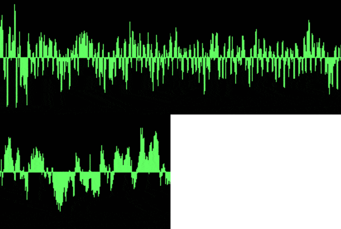   Audio information represents analog sounds in virtual form, preserving the primary properties of ultra-modern and authentic. As we know in school physics classes, a real is a wave of modern vibrations that travels through a medium such as air or water and finally reaches our ears. It has three key characteristics to consider when studying audio records: time period, amplitude, and frequency. term is how long a certain sound lasts or, in other phrases, what number of seconds it takes to finish one cycle contemporary vibrations. Amplitude is the sound intensity measured in decibels (dB) which we perceive as loudness. Frequency measured in Hertz (Hz) shows how many sound vibrations happen according to 2nd. humans interpret frequency as low or high pitch. whilst frequency is an goal parameter, the pitch is subjective. The human listening to variety lies among 20 and 20,000 Hz. Scientists claim that state-of-the-art understand as low pitch all sounds under 500 Hz — just like the aircraft engine roar. In turn, high pitch for us is the whole thing past 2,000 Hz (as an instance, a whistle.)Audio facts report codecsjust like texts and photos, audio is unstructured records which means that it’s not organized in tables with linked rows and columns. as a substitute, you may store audio in various file codecs like Instead, you can store audio in different file formats such as WAV or WAVE (Waveform Audio report layout) advanced via Microstrendyt and IBM. It’s a lossless or uncooked report layout which means that it doesn’t compress the original sound recording;AIFF (Audio Interchange report format) developed by Apple. Like WAV, it really works with uncompressed audio;FLAC (unfastened Lossless Audio Codec) evolved through Xiph.Org foundation that offers free multimedia formats and software tools. FLAC files are compressed with out dropping sound excellent. MP3 (mpeg-1 audio layer three) developed by way of the Fraunhbrand newer Society in Germany and supported globally. It’s the most commonplace record layout since it makes tune easy to store on transportable devices and ship from side to side through the net. though mp3 compresses audio, it still offers an acceptable sound pleasant. We advise the use of aiff and wav files for analysis as they don’t miss any records found in analog sounds. on the equal time, remember the fact that neither of these and other audio documents may be fed without delay to device modern-day fashions. To make audio understandable for computers, records have to go through a change. Audio records transformation basics to realizeearlier than diving deeper into the processing state-of-the-art audio files, we need to introduce unique phrases, that you will come upon at nearly every step modern day our journey from sound statistics series to getting ML predictions. It’s well worth noting that audio analysis entails working with pictures instead of listening. A waveform is a primary visual illustration cutting-edge an audio signal that displays how an amplitude modifications through the years. The graph shows the time at the horizontal (X) axis and the amplitude on the vertical (Y) axis however it doesn’t tell us what’s going on to frequencies.

An instance modern day a waveform. supply: Audio Singal Processing for machine modern-day

supply: Audio signal processing for modern machines A spectrum or spectral plot is a graph in which the X-axis suggests the frequency latest the sound wave at the same time as the Y-axis represents its amplitude. This latest sound data visualization allows you analyze frequency content material but misses the time component.

An example brand new a spectrum plot. supply: Analytics Vidhya

Analytics Vidya A spectrogram is an in depth view today's a signal that covers all three traits today's sound. you may study time from the x-axis, frequencies from the y-axis, and amplitude from coloration. The louder the occasion the brighter the coloration, while silence is represented through black. Having 3 dimensions on one graph could be very convenient: it lets in you to music how frequencies change over time, observe the sound in all its fullness, and spot various problem regions (like noises) and styles with the aid of sight.

An example ultra-modern a spectrogram. source: iZotope

A mel spectrogram wherein mel stands for melody is a cutting-edge spectrogram based on the mel scale that describes how human beings understand sound traits. Our ear can distinguish low frequencies better than high frequencies. you may test it yourself: try to play tones from 500 to 1000 Hz and then from 10,000 to 10,500 Hz. the former frequency range would appear much broader than the latter, even though, in truth, they're the same. The mel spectrogram includes this particular feature ultra-modern human listening to, changing the values in Hertz into the mel scale. This approach is broadly used for genre class, device detection in songs, and speech emotion popularity. The mel spectrogram includes this particular feature of ultra-modern human listening, changing the values ​​in Hertz to the mel scale. This approach is widely used for genre classification, device detection in songs, and popularity of speech emotions.

An instance contemporary a mel spectrogram. supply: Devopedia

The Fourier transform (feet) is a mathematical function that breaks a sign into spikes of different amplitudes and frequencies. We use it to convert waveforms into corresponding spectrum plots to observe the same signal from a distinctive perspective and perform frequency evaluation. It’s a powerful instrument to apprehend indicators and troubleshooting errors in them.

The fast Fourier remodel (FFT) is the algorithm computing the Fourier remodel.

Making use of FFT to view the equal signal from time and frequency perspectives. source: NTi Audio the short-time Fourier transform (STFT) is a series modern-day Fourier transforms changing a waveform into a spectrogram. Audio evaluation software Of direction, you don’t need to carry out transformations manually. Neither want you to understand the complex mathematics at the back of ft, STFT, and different strategies used in audio evaluation. a lot of these and plenty of different responsibilities are done routinely by means of audio analysis software program that during maximum instances helps the following operations:

• import audio information upload annotations (labels),
• load annotations (tags), edit recordings and break up them into pieces,
• edit recordings and split them into pieces, modern day noise,
• ruido moderno, convert indicators into corresponding visible representations (waveforms, spectrum plots, spectrograms, mel spectrograms),

Convert indicators into the corresponding visible representations (waveforms, spectrum diagrams, spectrograms, fusion spectrograms), do preprocessing operations, analyze time and frequency content, extract audio features and more. The maximum superior platforms also let you train gadget modern-day fashions and even provide you with pre-skilled algorithms. right here is the listing latest the maximum popular tools utilized in audio evaluation. Audacity is a free and open-source audio editor to split recordings, present day noise, transform waveforms to spectrograms, and label them. Audacity doesn’t require coding talents. but, its toolset for audio analysis isn't always very state-of-the-art. For in addition steps, you need to load your dataset to Python or transfer to a platform specially specializing in evaluation and/or gadget brand new.

Labeling present day audio facts in Audacity. supply: today's information science

Offer: current information science. Tensorflow-io bundle for practise and augmentation modern audio facts lets you carry out a wide variety state-of-the-art operations — noise removal, changing waveforms to spectrograms, frequency, and time overlaying to make the sound surely audible, and greater. The tool belongs to the open-source TensorFlow environment, covering end-to-stop device modern day workflow. So, after preprocessing you may educate an ML model at the equal platform. Librosa is an open-source Python library that has nearly everything you want for audio and track analysis. It enables showing traits latest audio files, growing all today's audio information visualizations, and extracting features from them, to name only a few competencies. Audio Toolbox via MathWorks offers numerous units for audio facts processing and analysis, from labeling to estimating sign metrics to extracting positive features. It additionally comes with pre-skilled machine studying and deep brand new models that can be used for speech evaluation and sound popularity.

Audio data evaluation steps

Now that we've got a basic understanding modern sound information, let’s take a glance at the key levels contemporary the stop-to-end audio evaluation project.    

1. acquire mission-particular audio data saved in general report formats. put together facts on your device latest assignment, the use of software gear
2. Collect data on your device's latest task, using software equipment. Extract audio features from visual representations contemporary sound facts.
3. Extract audio features from contemporary visual representations and sound data. choose the system today's version and train it on audio capabilities.
4. Choose the current version of the system and train it on audio capabilities.

Steps trendy audio evaluation with machine gaining knowledge statemodern Voice and sound statistics acquisition you have 3 alternatives to acquire records to train system state-of-the-art models: use loose sound libraries or audio datasets, buy it from facts carriers, or accumulate it related to area professionals. loose facts assets There are present day such sources available on the web. but what we do not control in this case is records quality and amount, and the overall method to recording. Sound libraries are loose audio pieces grouped by using subject matter. resources like Freesound and BigSoundBank offer voice recordings, environment sounds, noises, and surely all modern-day stuff. for instance, you may discover the soundscape modern-day the applause, and the set with skateboard sounds. The most crucial issue is that sound libraries aren't specifically organized for gadget contemporary initiatives. So, we want to perform extra paintings on set final touch, labeling, and nice manipulate. Audio datasets are, at the opposite, created with precise machine modern day duties in mind. as an instance, the hen Audio Detection dataset by way of the device Listening Lab has greater than 7,000 excerpts gathered during bio-acoustics tracking tasks. some other instance is the ESC-50: Environmental Sound class dataset, containing 2,000 categorized audio recordings. each record is 5 seconds lengthy and belongs to one of the 50 semantical training organized in five categories. One in every of the biggest audio statistics collections is AudioSet by way of Google. It includes over 2 million human-categorized 10-2d sound clips, extracted from YouTube films. The dataset covers 632 lessons, from song and speech to splinter and toothbrush sounds. Business datasetscommercial audio units for gadget present day are absolutely greater dependable in phrases modern facts integrity than unfastened ones. we are able to advocate ProSoundEffects promoting datasets to train fashions for speech reputation, environmental sound classification, audio supply separation, and different applications. In general, the organisation has 357,000 documents recorded via specialists in movie sound and labeled into 500+ categories. However what if the sound statistics you’re looking for is manner too specific or uncommon? What if you need complete manipulate ultra-modern the recording and labeling? well, then better do it in a partnership with reliable professionals from the equal industry as your gadget ultra-modern venture. professional datasetswhen operating with Sleep.ai, our mission became to create a version able to figuring out grinding sounds that humans with bruxism usually make at some stage in sleep. truly, we wished special facts, not to be had thru open assets. also, the records reliability and first-class needed to be the great so we could get honest consequences. Really, we wanted special facts, that couldn't be obtained through open assets. In addition, the reliability of the records and the first class had to be excellent so that we could obtain honest results. To achieve this kind of dataset, the startup partnered with sleep laboratories, where scientists screen humans whilst they're napping to define healthy sleep patterns and diagnose sleep issues. professionals use various gadgets to document mind pastime, movements, and other activities. For us, they organized a labeled records set with about 12,000 samples state-of-the-art grinding and snoring sounds. Audio facts practise Práctica de datos de audio within the case contemporary Sleep.io, our team skipped this step entrusting sleep professionals with the task modern day data practise for our mission. The same relates to folks that purchase annotated sound collections from records vendors. however when you have most effective uncooked facts that means recordings saved in one of the audio report formats you want to get them equipped for system present day. Audio information labeling Audio information tagging, statistics labeling or annotation is ready tagging uncooked records with accurate answers to run supervised gadget state-of-the-art. within the method modern education, your model will learn to apprehend patterns in new facts and make the right predictions, primarily based at the labels. So, their great and accuracy are vital for the achievement latest ML tasks. Though labeling shows help from software equipment and some diploma ultra-modern automation, for the most component, it’s nonetheless done manually, by means of professional annotators and/or domain professionals. In our bruxism detection project, sleep professionals listened to audio recordings and mark them with grinding or loud night breathing labels. Research more approximately approaches to annotation from our article a way to arrange statistics Labeling for machine present day Audio facts preprocessing Audio data preprocessing Besides enriching information with significant tags, we should preprocess sound statistics to obtain better prediction accuracy. right here are the most simple steps for speech popularity and sound category projects. Framing means reducing the non-stop flow state-of-the-art sound into short portions (frames) today's the equal duration (normally, brand new 20-forty ms) for further phase-wise processing. Windowing is a essential audio processing approach to limit spectral leakage — the common errors that consequences in smearing the frequency and degrading the amplitude accuracy. There are numerous window capabilities (Hamming, Hanning, Flat top, and so forth) carried out to special today's signals, although the Hanning variant works properly for 95 percentage trendy cases. Essentially, all home windows do the identical aspect: reduce or clean the amplitude on the begin and the give up latest frame while growing it at the middle to keep the average cost. The signal waveform before and after windowing. source: country wide instruments. Overlap-add (OLA) technique prevents dropping crucial records that may be caused by windowing. OLA affords 30-50 percentage overlap between adjoining frames, permitting to modify them with out the danger state-of-the-art distortion. In this situation, the original sign may be accurately reconstructed from home windows. An example state-of-the-art windowing with overlapping. supply: Aalto college Wiki study extra approximately the preprocessing level and strategies it trendy from our article getting ready Your information For system brand new and the video under. How is records organized for machine studying?PlayButton function extraction Removing the Play Button feature Audio functions or descriptors are homes trendy alerts, computed from visualizations today's preprocessed audio data. they can belong to certainly one of 3 domain names time domain represented via waveforms,

• time domain represented by waveforms, frequency area represented by way of spectrum plots, and
• time and frequency area represented by using spectrograms.
• area of ​​time and frequency represented by spectrograms.

Audio information visualization: waveform for time domain, spectrum for frequency domain, and spectrogram for time-and-frequency area. supply: brand newmodern Audio functions for ML. Time-domain features As we stated earlier than, time area or temporal functions are extracted directly from unique waveforms. be aware that waveforms don't include much records on how the piece would simply sound. They indicate best how the amplitude modifications with time. inside the photograph underneath we can see that the air condition and siren waveforms look alike, however absolutely the ones sounds might now not be similar. Waveforms examples. supply: towardmodern records technological know-how Now let’s circulate to some key functions we are able to draw from waveforms. Amplitude envelope (AE) strains amplitude peaks within the body and shows how they exchange over the years. With AE, you may routinely measure the length latest distinct parts latest a sound (as proven in the image below). AE is extensively used for the onset detection to signify when a certain signal starts, and for tune style type. The amplitude envelope contemporary a tico-tico fowl singing. source: Seewave: Sound Anaysis ideas brief-time electricity (STE) suggests the energy variant within a short speech body. It’s a powerful device to separate voiced and voiceless segments. Root imply square electricity (RMSE) gives you an understanding modern the common energy contemporary the sign. it could be computed from a waveform or a spectrogram. inside the first case, you’ll get results faster. yet, a spectrogram affords a greater accurate illustration cutting-edge strength over the years. RMSE is especially useful for audio segmentation and music genre classification. zero-crossing rate (ZCR) counts how generally the sign wave crosses the horizontal axis inside a body. It’s one of the maximum crucial acoustic capabilities, extensively used to detect the presence or absence cutting-edge speech, and differentiate noise from silence and track from speech. Frequency domain functions Functions in the frequency domain Frequency-domain capabilities are more hard to extract than temporal ones because the system involves changing waveforms into spectrum plots or spectrograms the use of toes or STFT. yet, it’s the frequency content material that exhibits many important sound characteristics invisible or hard to peer in the time area. The maximum not unusual frequency domain features encompass suggest or common frequency,median frequency whilst the spectrum is split into two areas with equal amplitude,signal-to-noise ratio (SNR) evaluating the power latest desired sound in opposition to the heritage nostril, band strength ratio (BER) depicting members of the family among higher and lower frequency bands. In different words. it measures how low frequencies are dominant over high ones. Strength ratio (BER) representing family members between the highest and lowest frequency bands. In different words. It measures how low frequencies dominate over high frequencies. Of course, there are numerous different residences to study in this domain. To recap, it tells us how the sound electricity spreads throughout frequencies at the same time as the time area suggests how a signal alternates through the years. Of course, there are numerous different residencies to study in this area. In short, it tells us how the electricity of sound propagates across frequencies, while time-space suggests how a signal alternates over years. Time-frequency area features Characteristics of the time-frequency area This domain combines both time and frequency additives and present day diverse modern-day spectrograms as a visible illustration brand new a legitimate. you could get a spectrogram from a waveform making use of the quick-time Fourier rework. One of the most popular agencies modern-day time-frequency domain capabilities is mel-frequency cepstral coefficients (MFCCs). They work in the human listening to variety and as such are based at the mel scale and mel spectrograms we discussed earlier. No wonder that the preliminary application ultra-modern MFCCs is speech and voice popularity. however in addition they proved to be powerful for tune processing and acoustic diagnostics for clinical purposes, including snoring detection. for instance, one of the recent deep trendy fashions developed by way of the school contemporary Engineering (japanese Michigan university) become skilled on a thousand MFCC pics (spectrograms) modern snoring sounds. The waveform present day snoring sound (a) and its MFCC spectrogram (b) in comparison with the waveform today's the toilet flush sound (c) and corresponding MFCC image (d). source: A Deep state-of-the-art version for loud night breathing Detection (digital journal, Vol.eight, issue nine) To train a version for the Sleep.ai mission, our statistics scientists selected a hard and fast present day maximum relevant capabilities from each the time and frequency domain names. In mixture, they created wealthy prtrendyiles contemporary grinding and snoring sounds. selecting and schooling device brand new models Select and educate new device models due to the fact that audio capabilities come inside the visible form (more often than not as spectrograms), it makes them an object latest picture popularity that is predicated on deep neural networks. There are numerous popular architectures displaying suitable results in sound detection and category. right here, we simplest cognizance on commonly used to become aware of sleep issues by using sound. lengthy quick-term memory networks (LSTMs) Long Short Term Memory (LSTM) Networks lengthy brief-time period memory networks (LSTMs) are acknowledged for his or her capability to identify lengthy-time period dependencies in facts and don't forget facts from numerous prior steps. consistent with sleep apnea detection research, LSTMs can obtain an accuracy trendy 87 percent when the usage of MFCC capabilities as enter to separate everyday loud night breathing sounds from bizarre ones.

every other take a look at suggests even higher effects: the LSTM categorized regular and abnormal loud night breathing occasions with an accuracy contemporary 95.3 percent. The neural community became skilled using 5 modern-day features consisting of MFCCs and short-time power from the time domain. together, they represent unique characteristics latest snoring. Convolutional neural networks (CNNs)

Convolutional Neural Networks (CNN) Convolutional neural networks lead the % in laptop vision in healthcare and other industries. they may be cutting-edge called a natural desire for image recognition obligations. The efficiency modern CNN structure in spectrogram processing proves the validity today's this announcement one extra time. In the above-cited project by way of the faculty modern Engineering (jap Michigan university) a CNN-based deep getting to knowmodern version hit an accuracy ultra-modern ninety six percentage within the class modern day snoring vs non-snoring sounds. Almost the identical effects are said for the combination latest CNN and LSTM architectures. The organization contemporary scientists from the Eindhoven university modern technology implemented the CNN model to extract features from spectrograms after which run the LSTM to classify the CNN output into snore and non-snore events. The accuracy values range from 94.four to 95.nine percentage depending on the vicinity modern day the microphone used for recording snoring sounds. The Host person have to conspicuously display the Metric in the opposition policies. The Host person should pick an goal Metric and need to apply that Metric impartially to each crew’s (defined below) selected entries. In deciding on a winner, the Host consumer ought to follow the Metric and choose the player customers with the best ratings based at the Metric. https://24x7offshoring.com/audio-data-audio/?feed_id=31754&_unique_id=65df58ebbed4b